Exercise 1: Topic modeling biodiversity preprints

This exercise follows the structure of the vignette("covid-preprint-topics") and adapts it to create a topic model for preprints referencing the term ‘biodiversity’ in either the preprint title or abstract. Refer back to the vignette("covid-preprint-topics") for more information about the individual steps.

Either try the steps yourself with the help of the example in the vignette("covid-preprint-topics") or jump ahead to the Solution section.

Exercise tasks

Getting the document data

We assume that you have created a local copy of the preprint data to run this analysis (see information and code samples for “Getting the document data” in vignette("covid-preprint-topics")).

load(url("PREPRINT_RDATA_LOCATION_HERE"))

Cleaning, filtering and annotating the data

For this example we are planning to explore whether the publication status influences the topic prevalence. We therefore adapt the time range and consider preprints added from 2017 to 2021. We then reduce this to a subset of preprints that reference the term ‘biodiversity’ in either the preprint title or abstract.

# adapt based on the covid preprints example

Preparing and preprocessing the documents for text analysis

Create a corpus

Create a corpus and explore its properties.

# quanteda is used for corpus creation

Tokenize and preprocess

Tokenize by applying the same steps as in the Covid preprint example.

# quanteda is used for tokenization

Create a Document-feature matrix

# quanteda is used for creation of a DFM 

Filter terms and documents

Remove stopwords from the document-feature-matrix. Explore its properties.

# quanteda is used for stopword removal 

Filter tokens and documents by applying the same approach as in the Covid preprint example.

# quanteda is used for filtering

Topic modeling

Fitting the STM topic model

Fit an stm topic model with 10 topics to the prepared data. The model should consider an interacting effect between the covariates is_published and publication year on topical prevalence. Apply a seed argument with the value 9868467.

# convert the DFM into stm format and run the stm() function

Estimating the effect of document covariates

Evaluate the effect of the previously chosen topic prevalence covariates on all topics.

# estimateEffect() on the topic model

This concludes fitting the model. The following sections step through a sample exploration of this topic model.

Analysing and interpreting the topic model

Basic topic model information

Plot a model summary with the 7 most frequent words per topic.

# stm plot() teh topic model provides a summary of topic proportions

Print a summary() of the topic model and explore the sets of words that characterize the 10 topics.

# print a summary() of the topic model

Understanding and labeling topics

Create word clouds for all 10 topics using the 30 words with the highest probability per topic. Remove the term “biodiversity” from this display.

# word clouds are a useful first step to arrive at summary labels for topics

Covariate effects

Print the regression tables for all or selected topics.

# print a summary() of effects

Publication year

Use the stm plot method to create a plot that shows the effect of publication year on topical prevalence for Topic 4 and Topic 8. Annotate with the most probable terms.

# stm plot offers various different plot options for covariate effects

Alternatively, the stminsights package could be used to extract the same regression information from the stm effects object and create customized charts.

# stminsights allows to get effects in a format suitable for ggplot2

Publication status effect

We also incoporated the publication status into the model (covariate is_published). Using the stm plot method explore the effect of the treatment “published” on topical prevalence.

# stm plot offers various different plotoptions for covariate effects

Compare the topical prevalence effect of covariate is_published for Topic 4.

# stm plot offers various different plotoptions for covariate effects

Combination of publication status and publication year

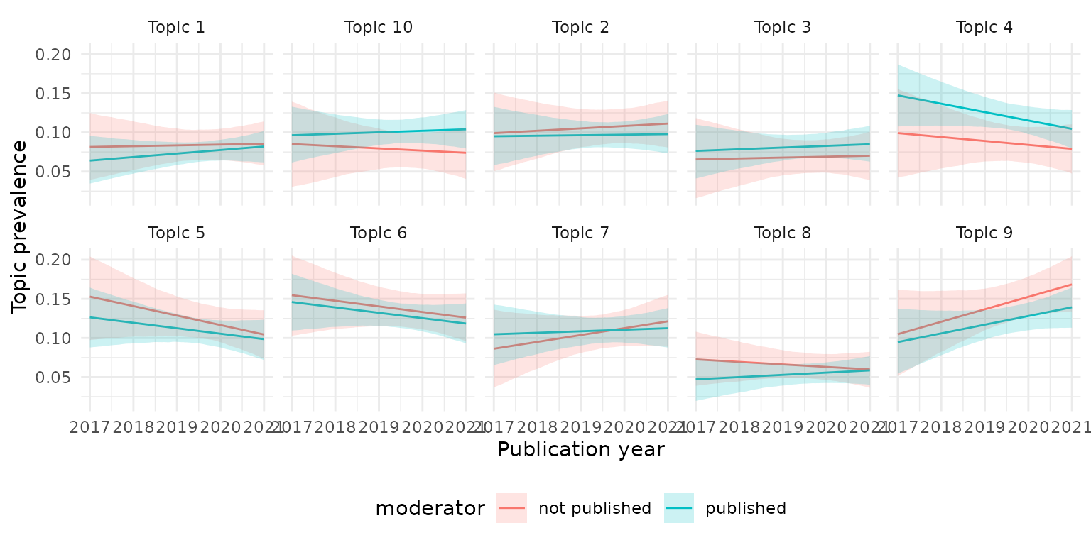
Finally, we can also explore the combined effect of covariates; we assumed an interacting effect of the two covariates is_published and year. Using the stm plot function explore the combined interacting covariate effect for Topic 4.

Again, stminsights can be used to retrieve this information and create customized visualizations for the combined covariate effect.

# stminsights allows to get effects in a format suitable for ggplot2

Exploring the topic structure

Topic correlations

Finally, retrieve the topic correlations matrix and plot a cooccurrence network.

# topic correlations retrieved with stm

Solution

Getting the document data

We assume that you have created a local copy of the preprint data to run this analysis (see information and code samples for “Getting the document data” in vignette("covid-preprint-topics")).

load(url("PREPRINT_RDATA_LOCATION_HERE"))

Cleaning, filtering and annotating the data

For this example we are planning to explore whether the publication status influences the topic prevalence. We therefore adapt the time range and consider preprints added from 2017 to 2021. We then reduce this to a subset of preprints that reference the term ‘biodiversity’ in either the preprint title or abstract.

library(dplyr)
library(stringr)

preprints_cleaned <- preprints_raw %>%
  group_by(doi) %>%
  filter(version == max(version)) %>%
  ungroup() %>%
  distinct(doi, .keep_all = TRUE)

preprints <- preprints_cleaned %>%
  mutate(published = stringr::str_trim(published)) %>%
  mutate(published = na_if(published, "NA")) %>%
  mutate(is_published = as.numeric(!is.na(published))) %>%
  mutate(is_published = case_when(is_published == 1 ~ "published",
                                  is_published == 0 ~ "not published",
                                  TRUE ~ "undefined")) %>%
  mutate(year = lubridate::year(date)) %>%
  filter(year >= 2017 & year <= 2021) %>% 
  select(doi, server, title, abstract, date, year, version, is_published)

keywords <- c("biodiversity")

search_pattern <- stringr::regex(paste(keywords, collapse = "|"), 
                                 ignore_case = TRUE)

biodiv_preprints <- preprints %>%
  filter(stringr::str_detect(title, pattern = search_pattern) |
           stringr::str_detect(abstract, pattern = search_pattern))

Preparing and preprocessing the documents for text analysis

Create a corpus

Create a corpus and explore its properties.

library(quanteda)

pubs_corpus <- biodiv_preprints %>%
  quanteda::corpus(docid_field = "doi", text_field = "abstract")

# pubs_corpus
# Corpus consisting of 29,692 documents and 6 docvars.

Tokenize and preprocess

Tokenize by applying the same steps as in the Covid preprint example.

pubs_tokens <- pubs_corpus %>%
  quanteda::tokens(remove_punct = TRUE,
                   remove_symbols = TRUE,
                   remove_numbers = TRUE,
                   remove_url = TRUE,
                   remove_separators = TRUE,
                   split_hyphens = TRUE) 

Create a Document-feature matrix

pubs_dfm <- pubs_tokens %>%
  quanteda::dfm()

Filter terms and documents

Remove stopwords from the document-feature-matrix. Explore its properties.

pubs_dfm <- pubs_dfm %>%
  quanteda::dfm_remove(pattern = quanteda::stopwords("english")) #%>%
  #quanteda::dfm_wordstem()

Filter tokens and documents by applying the same approach as in the Covid preprint example.

pubs_dfm <- pubs_dfm %>%
  quanteda::dfm_remove(min_nchar = 2) %>%
  quanteda::dfm_trim(min_docfreq = 2, docfreq_type = "count") %>%
  quanteda::dfm_subset(quanteda::ntoken(.) > 4)

Topic modeling

Fitting the STM topic model

Fit an stm topic model with 10 topics to the prepared data. The model should consider an interacting effect between the covariates is_published and publication year on topical prevalence. Apply a seed argument with the value 9868467.

library(stm)

biodiv_stm_docs <- quanteda::convert(pubs_dfm, to = "stm")

biodiv_model_K10 <- stm(documents = biodiv_stm_docs$documents,
                    vocab = biodiv_stm_docs$vocab,
                    data = biodiv_stm_docs$meta,
                    prevalence = ~ is_published * year,
                    K = 10,
                    verbose = TRUE,
                    seed = seed_stm)

Estimating the effect of document covariates

Evaluate the effect of the previously chosen topic prevalence covariates on all topics.

biodiv_effect_K10 <- estimateEffect(1:10 ~ is_published * year,
                                   stmobj = biodiv_model_K10,
                                   metadata = biodiv_stm_docs$meta)

This concludes fitting the model. The following sections step through a sample exploration of this topic model.

Analysing and interpreting the topic model

Basic topic model information

Plot a model summary with the 7 most frequent words per topic.

plot(biodiv_model_K10, n = 7)

Print a summary() of the topic model and explore the sets of words that characterize the 10 topics.

summary(biodiv_model_K10)
># A topic model with 10 topics, 1495 documents and a 8838 word dictionary.
># Topic 1 Top Words:
>#       Highest Prob: species, fish, marine, invasive, biodiversity, native, river 
>#       FREX: coral, reefs, lakes, fisheries, reef, fishing, ocean 
>#       Lift: advection, afdw, aggregations, aleutian, ampat, amphipods, andaman 
>#       Score: fish, reef, islands, coral, fisheries, fishing, sea 
># Topic 2 Top Words:
>#       Highest Prob: data, species, biodiversity, can, information, using, research 
>#       FREX: user, users, automated, learning, databases, images, algorithms 
>#       Lift: cheilostome, cnns, crux, digitized, disparities, dnn, echolocating 
>#       Score: images, users, user, algorithms, pipeline, learning, students 
># Topic 3 Top Words:
>#       Highest Prob: host, disease, biodiversity, populations, microbiota, human, infection 
>#       FREX: infection, pathogen, virus, viruses, viral, diseases, infections 
>#       Lift: antimicrobial, antimicrobials, attack, auxiliary, baits, brain, brood 
>#       Score: infection, disease, host, pathogen, gut, microbiota, virus 
># Topic 4 Top Words:
>#       Highest Prob: genetic, species, genome, populations, gene, population, genes 
>#       FREX: snp, alleles, introgression, genome, genomic, genetic, genomes 
>#       Lift: 3a, admixed, angustifolia, antibacterial, aureus, beak, beast 
>#       Score: genome, genetic, genes, genomes, genomic, gene, speciation 
># Topic 5 Top Words:
>#       Highest Prob: species, model, biodiversity, can, ecological, models, dynamics 
>#       FREX: coexistence, competitive, theory, simulations, competition, stability, empirical 
>#       Lift: abandon, absences, accumulates, aggressively, anchovy, archosaurs, assumes 
>#       Score: competitive, theory, coexistence, competition, stability, simulations, preemption 
># Topic 6 Top Words:
>#       Highest Prob: species, diversity, biodiversity, change, richness, climate, across 
>#       FREX: climatic, gradients, biotic, turnover, climate, scales, richness 
>#       Lift: arabia, bioregions, bryophyte, constantly, divide, endotherms, equivalence 
>#       Score: richness, climate, elevational, phylogenetic, zeta, ldg, gradients 
># Topic 7 Top Words:
>#       Highest Prob: plant, soil, diversity, communities, microbial, community, species 
>#       FREX: mixtures, fire, soil, aboveground, amf, nitrogen, plant 
>#       Lift: biodiv, conditioned, decomposer, exudate, fertilisation, microclimate, microsite 
>#       Score: soil, microbial, grazing, bacterial, amf, mixtures, crop 
># Topic 8 Top Words:
>#       Highest Prob: forest, forests, species, tree, cover, de, biodiversity 
>#       FREX: forest, forests, en, de, plantations, la, es 
>#       Lift: como, diversidad, landcover, que, una, vegetable, acacia 
>#       Score: forest, forests, la, que, de, las, plantations 
># Topic 9 Top Words:
>#       Highest Prob: conservation, species, biodiversity, areas, land, use, management 
>#       FREX: iucn, socio, protected, lands, pas, conservation, nations 
>#       Lift: eu, herpetofauna, pas, 30x30, abroad, accessing, achievements 
>#       Score: protected, land, pas, iucn, lands, natura, conservation 
># Topic 10 Top Words:
>#       Highest Prob: dna, edna, samples, species, metabarcoding, biodiversity, diversity 
>#       FREX: edna, metabarcoding, samples, dna, primer, coi, biomonitoring 
>#       Lift: 1the, acuta, asv, battery, benthos, bony, bruv 
>#       Score: edna, metabarcoding, dna, samples, primer, coi, cristatus

Understanding and labeling topics

Create word clouds for all 10 topics using the 30 words with the highest probability per topic. Remove the term “biodiversity” from this display.

library(tidyr)
library(tibble)

# get the top FREX words
frex_top20 <- as.data.frame(labelTopics(biodiv_model_K10, n = 25)$frex) %>%
  rownames_to_column(var = "topic") %>%
  pivot_longer(starts_with("V"), values_to = "term") %>%
  mutate(is_frex = 1) %>%
  select(-name)

topic_words <- tidytext::tidy(biodiv_model_K10, matrix = "beta") %>%
  #filter(!(term %in% c("sars", "cov", "covid"))) %>% 
  mutate(topic = as.character(topic)) %>%
  group_by(topic) %>%
  arrange(-beta) %>%
  slice_head(n = 30) %>%
  mutate(beta_norm = (beta - min(beta)) / (max(beta) - min(beta))) %>%
  ungroup() %>%
  left_join(frex_top20, by = c("topic", "term")) %>%
  mutate(is_frex = ifelse(is.na(is_frex), "0", "1")) %>%
  filter(!(term %in% c("biodiversity"))) %>%
  mutate(topic = paste("Topic", topic))

ggplot(topic_words, aes(label = term, size = beta_norm, color = is_frex)) +
  ggwordcloud::geom_text_wordcloud_area(shape = "square",
                                        family = "Arial",
                                        rm_outside = TRUE) +
  scale_radius(range = c(4, 15)) +
  scale_color_manual(values = c("0" = "black", "1" = "#D55E00")) + 
  facet_wrap(~topic, ncol = 5)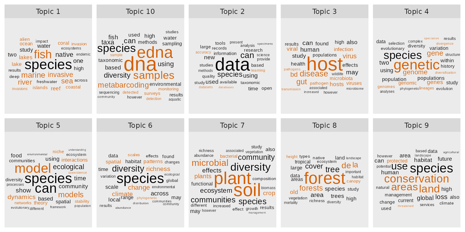

Word clouds showing the 30 most probable terms per topic.

Covariate effects

Print the regression tables for all or selected topics.

summary(biodiv_effect_K10)
># 
># Call:
># estimateEffect(formula = 1:10 ~ is_published * year, stmobj = biodiv_model_K10, 
>#     metadata = biodiv_stm_docs$meta)
># 
># 
># Topic 1:
># 
># Coefficients:
>#                              Estimate Std. Error t value Pr(>|t|)
># (Intercept)                -1.5640291 15.0326886  -0.104    0.917
># is_publishedpublished      -7.0301857 19.4839231  -0.361    0.718
># year                        0.0008161  0.0074433   0.110    0.913
># is_publishedpublished:year  0.0034767  0.0096470   0.360    0.719
># 
># 
># Topic 2:
># 
># Coefficients:
>#                             Estimate Std. Error t value Pr(>|t|)
># (Intercept)                -5.864350  17.558532  -0.334    0.738
># is_publishedpublished       4.770673  23.180684   0.206    0.837
># year                        0.002957   0.008694   0.340    0.734
># is_publishedpublished:year -0.002367   0.011477  -0.206    0.837
># 
># 
># Topic 3:
># 
># Coefficients:
>#                             Estimate Std. Error t value Pr(>|t|)
># (Intercept)                -2.002719  18.120082  -0.111    0.912
># is_publishedpublished      -2.117502  22.815117  -0.093    0.926
># year                        0.001026   0.008972   0.114    0.909
># is_publishedpublished:year  0.001055   0.011297   0.093    0.926
># 
># 
># Topic 4:
># 
># Coefficients:
>#                             Estimate Std. Error t value Pr(>|t|)
># (Intercept)                 9.944577  19.120834   0.520    0.603
># is_publishedpublished      12.356281  23.648316   0.523    0.601
># year                       -0.004881   0.009467  -0.516    0.606
># is_publishedpublished:year -0.006102   0.011709  -0.521    0.602
># 
># 
># Topic 5:
># 
># Coefficients:
>#                              Estimate Std. Error t value Pr(>|t|)
># (Intercept)                 24.355948  18.649238   1.306    0.192
># is_publishedpublished      -10.386704  23.575235  -0.441    0.660
># year                        -0.012000   0.009234  -1.300    0.194
># is_publishedpublished:year   0.005136   0.011673   0.440    0.660
># 
># 
># Topic 6:
># 
># Coefficients:
>#                              Estimate Std. Error t value Pr(>|t|)
># (Intercept)                 1.445e+01  1.738e+01   0.832    0.406
># is_publishedpublished      -2.035e-01  2.231e+01  -0.009    0.993
># year                       -7.089e-03  8.603e-03  -0.824    0.410
># is_publishedpublished:year  9.688e-05  1.105e-02   0.009    0.993
># 
># 
># Topic 7:
># 
># Coefficients:
>#                              Estimate Std. Error t value Pr(>|t|)
># (Intercept)                -17.687078  18.700595  -0.946    0.344
># is_publishedpublished       13.866209  23.293191   0.595    0.552
># year                         0.008812   0.009259   0.952    0.341
># is_publishedpublished:year  -0.006865   0.011534  -0.595    0.552
># 
># 
># Topic 8:
># 
># Coefficients:
>#                              Estimate Std. Error t value Pr(>|t|)
># (Intercept)                  6.844616  12.808529   0.534    0.593
># is_publishedpublished      -12.253607  16.051870  -0.763    0.445
># year                        -0.003357   0.006342  -0.529    0.597
># is_publishedpublished:year   0.006063   0.007948   0.763    0.446
># 
># 
># Topic 9:
># 
># Coefficients:
>#                              Estimate Std. Error t value Pr(>|t|)  
># (Intercept)                -32.127319  19.311673  -1.664   0.0964 .
># is_publishedpublished        9.886685  25.146786   0.393   0.6943  
># year                         0.015980   0.009562   1.671   0.0949 .
># is_publishedpublished:year  -0.004906   0.012451  -0.394   0.6936  
># ---
># Signif. codes:  0 '***' 0.001 '**' 0.01 '*' 0.05 '.' 0.1 ' ' 1
># 
># 
># Topic 10:
># 
># Coefficients:
>#                             Estimate Std. Error t value Pr(>|t|)
># (Intercept)                 5.787510  18.035606   0.321    0.748
># is_publishedpublished      -9.518606  21.515554  -0.442    0.658
># year                       -0.002827   0.008930  -0.317    0.752
># is_publishedpublished:year  0.004725   0.010653   0.444    0.657

Publication year

Use the stm plot method to create a plot that shows the effect of publication year on topical prevalence for Topic 4 and Topic 8. Annotate with the most probable terms.

plot(biodiv_effect_K10,
     covariate = "year",
     method = "continuous",
     model = biodiv_model_K10,
     topics = c(4, 8),
     xaxt = "n",
     main = 'Effect of publication year on prevalence of Topic 4 ("???") and Topic 8 ("???")',
     labeltype = "prob",
     xlab = "Publication year")
axis(1, at = c("2017","2018","2019","2020", "2021"), labels = c(2017, 2018, 2019, 2020, 2021))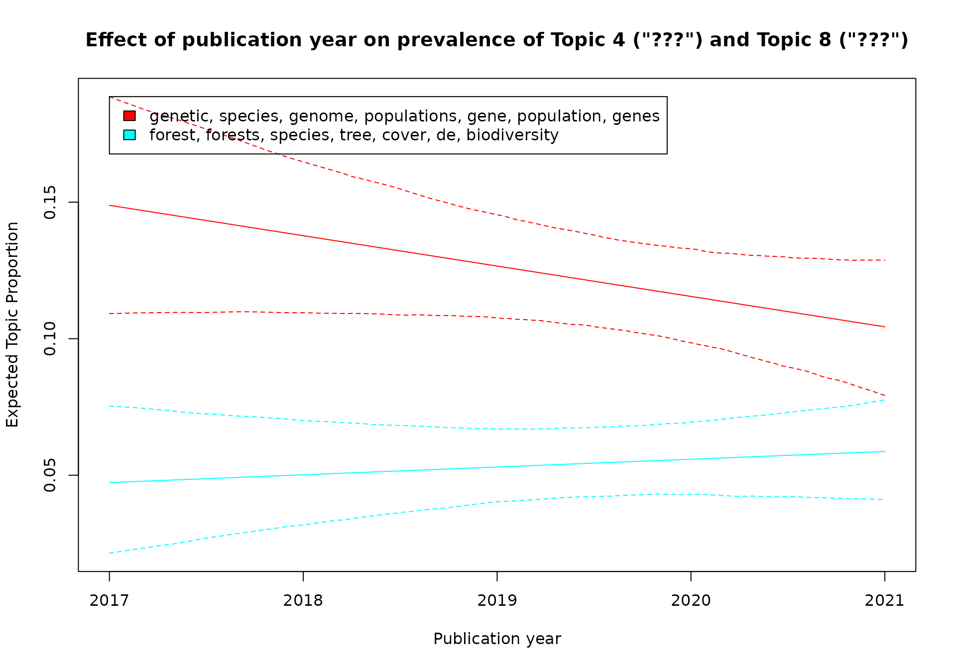

Alternatively, the stminsights package could be used to extract the same regression information from the stm effects object and create customized charts.

library(stminsights)

year_effect <- get_effects(estimates = biodiv_effect_K10, 
                           variable = "year",
                           type = "continuous")

year_effect %>%
  mutate(topic = as.character(topic)) %>%
  mutate(topic = paste("Topic", topic)) %>%
    ggplot(aes(x = value, y = proportion)) +
      geom_line() +
      geom_ribbon(aes(ymin = lower, ymax = upper), 
                  alpha = 0.2, linetype = 0)  +
      xlab("Publication year") +
      ylab("Topic prevalence") +
      facet_wrap(~topic, ncol = 5) +
      theme_minimal()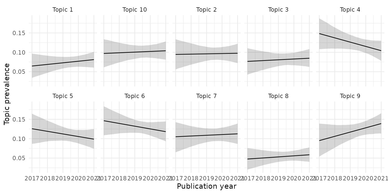

Publication status effect

We also incoporated the publication status into the model (covariate is_published). Using the stm plot method explore the effect of the treatment “published” on topical prevalence.

plot(biodiv_effect_K10, 
     covariate = "is_published",
     #topics = c(9, 10, 16, 1),
     model = biodiv_model_K10, 
     method = "difference",
     cov.value1 = "published", cov.value2 = "not published",
     xlab = "higher prevalence in unpublished ... higher prevalence in published",
     #xlim = c(-0.19, 0.1),
     #labeltype = "prob",
     main = "Effect of preprint server (treatment 'published')")

Compare the topical prevalence effect of covariate is_published for Topic 4.

plot(biodiv_effect_K10, 
     covariate = "is_published",
     topics = c(4),
     model = biodiv_model_K10, 
      method = "pointestimate",
     xlab = "Topical prevalence",
     #xlim = c(-0.04, 0.2),
     #labeltype = "prob",
     main = "Effect of preprint 'is_published' covariate for Topic 4")

Combination of publication status and publication year

Finally, we can also explore the combined effect of covariates; we assumed an interacting effect of the two covariates is_published and year. Using the stm plot function explore the combined interacting covariate effect for Topic 4.

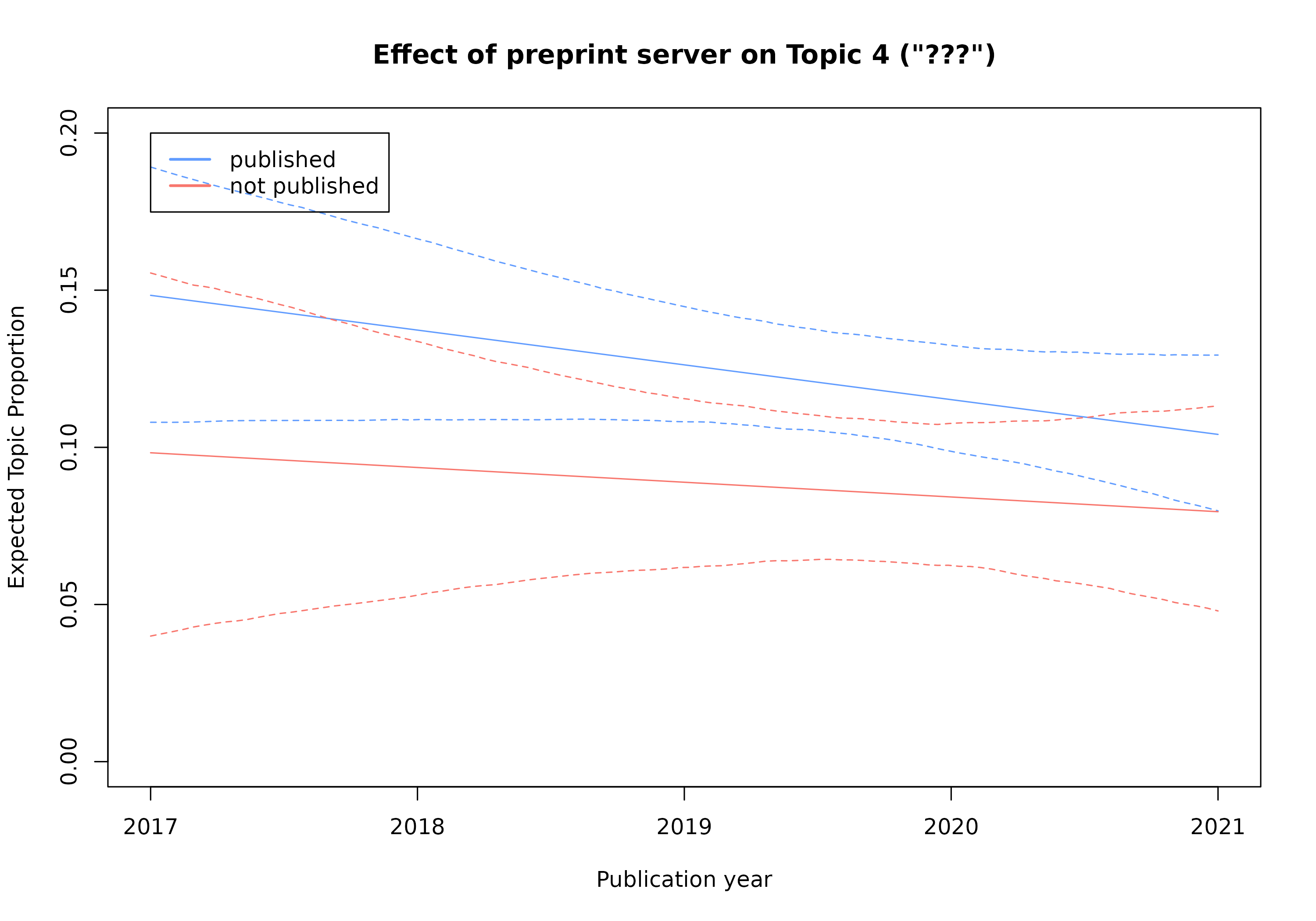
Again, stminsights can be used to retrieve this information and create customized visualizations for the combined covariate effect.

published_effect <- get_effects(biodiv_effect_K10, 
                                variable = "year", type = "continuous", 
                                moderator = "is_published", modval = "published")

unpublished_effect <- get_effects(biodiv_effect_K10,
                                  variable = "year", type = "continuous", 
                                  moderator = "is_published", modval = "not published")

is_published_effects <- bind_rows(published_effect, unpublished_effect)

is_published_effects %>%
  mutate(topic = as.character(topic)) %>%
  mutate(topic = paste("Topic", topic)) %>%
    ggplot(aes(x = value, y = proportion, color = moderator,
               group = moderator, fill = moderator)) +
      geom_line() +
      geom_ribbon(aes(ymin = lower, ymax = upper, 
                      fill = moderator), alpha = 0.2, linetype = 0) +
      xlab("Publication year") +
      ylab("Topic prevalence") +
      facet_wrap(~topic, ncol = 5) +
      theme_minimal() +
      theme(legend.position = "bottom") 

Exploring the topic structure

Topic correlations

Finally, retrieve the topic correlations matrix and plot a cooccurrence network.

covid_topic_correlations <- topicCorr(biodiv_model_K10, cutoff = 0.001)

plot(covid_topic_correlations)