Markdown

Markdown allows us to concentrate on document structure and content. We can then worry about styling and presentation later.

RMarkdown

• Purpose: dynamically weave together text, data and analysis workflows.
• This is accomplished with the knitr package, an R package conveniently integrated into the R Studio UI.

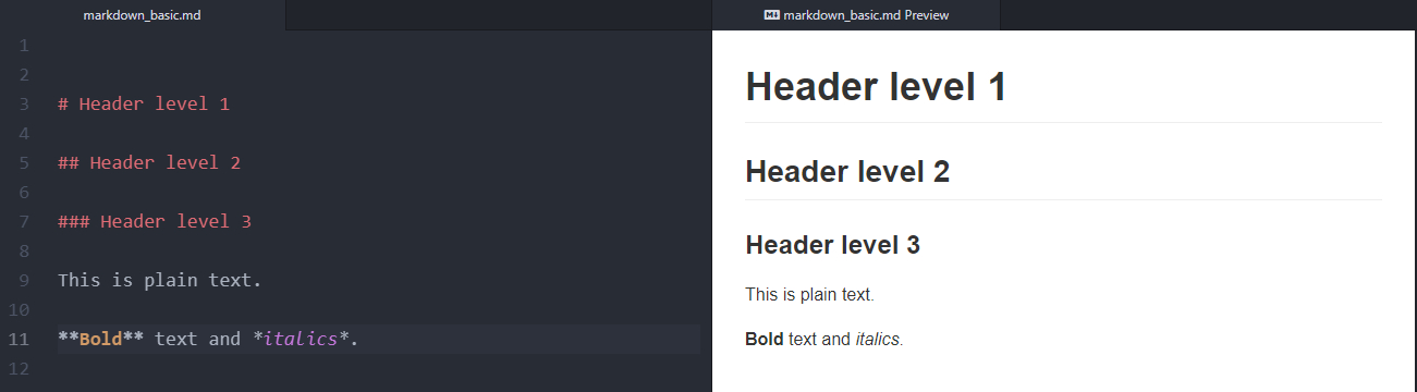
Sample Markdown

# Top-level header

## Second-level header

This is a list:

* with some **bold** and 
* some *italic* text.

And a [hyperlink](https://bookdown.org/yihui/rmarkdown/) for good measure.

Basic formatting and structuring

RMarkdown: data-driven documents!

• Analysis can be integrated as R code into the document
• The analysis (i.e. the R code) is executed and the results updated when you knit the document.
• Text and code are interspersed.
• Code sections are included in code chunks like this.

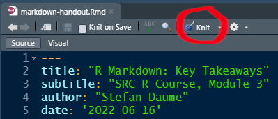
The ‘YAML’ header

The YAML header must be placed at the beginning of a document and is enclosed by three dashes ---.

---
title: "Untitled"
output: html_document
date: '2022-12-16'
---

Above is the default YAML header when generating an RMarkdown file in R Studio.

Translating RMarkdown to HTML, PDF, Word etc

Turning RMarkdown into a shiny app

---
title: "Untitled"
output: html_document
date: '2022-12-16'
runtime: shiny
---

Now “knit” is replaced by “run”

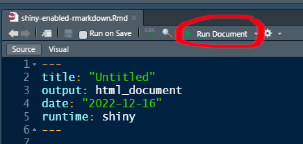
And you need the “app logic”

Which will be included in the code chunks of the R Markdown document.

Create a sample interactive R Markdown document

In RStudio select: File > New File > R Markdown

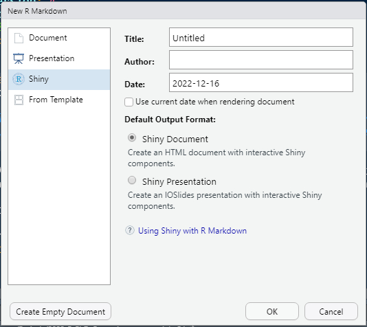
Default example

Interactive code in the default example

```{r eruptions, echo=FALSE}
inputPanel(
  selectInput("n_breaks", label = "Number of bins:",
              choices = c(10, 20, 35, 50), selected = 20),
  
  sliderInput("bw_adjust", label = "Bandwidth adjustment:",
              min = 0.2, max = 2, value = 1, step = 0.2)
)

renderPlot({
  hist(faithful$eruptions, probability = TRUE, breaks = as.numeric(input$n_breaks),
       xlab = "Duration (minutes)", main = "Geyser eruption duration")
  
  dens <- density(faithful$eruptions, adjust = input$bw_adjust)
  lines(dens, col = "blue")
})
```

Change the output format to flex_dashboard

Example

Change the layout

Dashboards are composed of rows and columns. Each output component is indicated by a level 3 header (i.e. ###).

• turn all sections into components
• change the flex_dashboard layout to vertical

---
title: "Untitled"
output: 
  flexdashboard::flex_dashboard:
    vertical_layout: scroll
date: "2022-12-16"
runtime: shiny
---

Example

Split input and output logic into different “components”

Example

Change the component layout

flexdashboard allows flexible layouts that are basically controlled through markdown section headers at three levels.

• create two separate dash board pages by adding a level 1 markdown section header above the first two and the last “components” respectively. Both the header variant # and =========================== will work.

Example

Create a nested layout for the first page

Place the “Inputs” and “Outputs” sections next to each other. This can be achieved by adding a level 2 markdown section header named Column above each of these sections. Both the header variant ## and ----------------------- will work.

Example

Change the dashboard theme and add

flexdashboard offers flexible styling of the output. Several built-in themes can be applied via the YAML header.

Example

and more options …

There is a broad range of styling options and components that can be controlled via the YAML header and standard R Markdown elements.

Example

Key Resources

• R Markdown
  • R Markdown: The Definitive Guide (Xie, Allaire, and Grolemund 2022)
  • Cheatsheet: Dynamic documents with rmarkdown cheatsheet
• Git/Github:
  • Happy Git and GitHub for the useR (Bryan 2021)
  • “Excuse me, do you have a moment to talk about version control?” (Bryan 2017)
  • Advanced git use: Pro Git book (Chacon and Straub 2014)
  • How to write a great commit message

References

Bryan, Jennifer. 2017. “Excuse me, do you have a moment to talk about version control?” PeerJ Preprints 5:e3159v2 (August). https://doi.org/10.7287/PEERJ.PREPRINTS.3159V2.
———. 2021. “Happy Git and GitHub for the useR.” https://happygitwithr.com/.
Chacon, Scott, and Ben Straub. 2014. Pro Git. Apress. https://doi.org/10.1007/978-1-4842-0076-6.
Xie, Yihui, J. J. Allaire, and Garrett Grolemund. 2022. “R Markdown: The Definitive Guide.” https://bookdown.org/yihui/rmarkdown/.
Colophon
SRC PhD R course Module 7 — Interactive R Markdown with Shiny" by Stefan Daume
Presented on 16. December 2022.
This presentation can be cited using: doi:…
PRESENTATION DETAILS
Author/Affiliation: Stefan Daume, Stockholm Resilience Centre, Stockholm University
Presentation URL: https://sdaume.github.io/r-course-module-3/slides/shiny-module.html
Presentation Source: [TBD]
Presentation PDF: [TBD]
CREDITS & LICENSES
This presentation is delivered with the help of several free and open source tools and libraries. It utilises the reveal.js presentation framework and has been created using RMarkdown, knitr, RStudio and Pandoc. highlight.js provides syntax highlighting for code sections. MathJax supports the rendering of mathematical notations. PDF and JPG copies of this presentation were generated with DeckTape. Please note the respective licenses of these tools and libraries.
If not noted and attributed otherwise, the contents (text, charts, images) of this presentation are Copyright © 2022 of the Author and provided under a CC BY 4.0 public domain license.